


Abstract
In traditional pharmacokinetic models, blood flow or liquid transit is often expressed as first-order kinetics. When the flow expression by first-order kinetics is used for dynamic simulation, the flow velocity illogically depends on the step size of a solver of ordinary differential equations. In this study, we propose flow modeling using hybrid automata that combine ordinary differential equations and recursive equations, and we have preliminarily applied the constructed models to several examples. The blood concentration–time profiles of p-aminohippurate and propranolol after intravenous administration were successfully reproduced by simple hybrid automata. The simulation results of one-dimensional tube flow have demonstrated that the fluid velocity in the hybrid automata was independent of the step size of the ordinary differential equation solver. A body fluid model coordinated various flows in a human body with scheduled daily activities and could be used as a drug container to describe formulation-dependent disposition of 5-aminosalicylic acid and enterohepatic circulation of a virtual drug. These findings suggested that flow modeling using hybrid automata could avoid the logical inconsistency in the traditional pharmacokinetic modeling and that the hybrid automata have high versatility and a wide range of applicability to pharmacokinetic analysis. Because our method can define various intervals for multiple recursive equations, the resolution of a specific part of a model can be adjusted relatively freely while the whole body is being roughly modeled, which would be beneficial to refine a coarse model into a fine model in future.
SIGNIFICANCE STATEMENT There is a logical inconsistency in flow expression by first-order kinetics in ordinary differential equations used in traditional pharmacokinetic modeling. It is difficult to model a whole human body using flow models in partial differential equations because of the excessive calculation costs. Our simulations on tube flow and body fluids have demonstrated that the flow modeling using hybrid automata could avoid the problems. The preliminary applications of hybrid automata to several examples highlighted its high versatility in pharmacokinetic analysis.
Introduction
In pharmacokinetic theory, there are several ways to express blood flow or liquid transit in a human body. The well stirred model, which is traditionally used, defines both blood flow and intrinsic clearance as first-order kinetics in an ordinary differential equation (ODE) for drug concentration, and its organ clearance (CLorg) is expressed by eq. 1 (Rowland et al., 1973):
 where Q is the blood flow rate, fu,b is the fraction of unbound drug in the blood, and CLint is intrinsic clearance. Physiologically based pharmacokinetic (PBPK) models, which are often used for dynamic analysis to predict drug disposition, also adopt first-order kinetics in ODEs to connect compartments with blood flow or liquid transit. A tank-in-series model, which deploys multiple in-line well stirred compartments (Saville et al., 1992), or a combination of tank-in-series models are often used to express organs in a PBPK model. For example, it has been reported that a model in which the liver was composed of five compartments produced the value of availability most similar to that produced by a dispersion model with DN = 0.17 (Iga et al., 2006; Watanabe et al., 2009). Similarly, for other organ models such as intestine and kidney, the compartments are connected in line by the first-order kinetics (Yu et al., 1996; Jamei et al., 2009; Burt et al., 2016; Li et al., 2018; Nishiyama et al., 2019).
The parallel-tube model expresses blood flow as one-dimensional convection in a partial differential equation (PDE) with an axis in the flow direction (Pang and Rowland, 1977), and its organ clearance is expressed by eq. 2:

The dispersion model is also defined as a PDE and considers the axial dispersion addition to the convection (Roberts and Rowland, 1986a), and its organ clearance is expressed by eq. 3:
 where DN is dispersion number. It is known that a value of DN = 0.17 best describes the observed hepatic availability (Roberts and Rowland, 1986b).
There is a logical inconsistency derived from expressing liquid flow as first-order kinetics, although the flow models based on the first-order kinetics in ODEs are easy to handle in dynamic simulations. The flow based on the first-order kinetics in ODEs indicates that a part of the fluid in a compartment moves a finite distance from the compartment to the next in an infinitesimal time, leading to the infinite velocity of the fluid (Supplemental Fig. 1A). When those models are discretized for simulation, the flow velocity depends on the step size of an ODE solver. With a small step size, most of the compartment volume does not flow despite being expressed as a flow, whereas the flowing volume exceeds the volume existing in a compartment with a large step size (Supplemental Fig. 1A). Although the flow models in PDEs do not suffer from this logical inconsistency (Supplemental Fig. 1B), it is difficult to model a whole human body finely because of the excessive calculation costs as the result of too large model size.

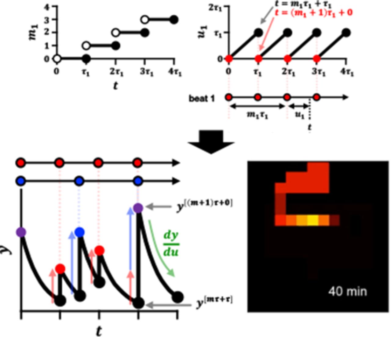
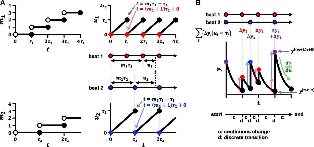
The concept of calculation for hybrid automata with multiple beats. (A) Time t is expressed by m and u in each beat. (B) By overlaying multiple beats on the t-axis, a hybrid automaton alternates continuous changes and discrete transitions.
To avoid the logical inconsistency in the ODE flow models and the difficulty in the size of the PDE models at the same time, we propose another flow modeling using hybrid automata that combine ODEs and recursive equations. The hybrid automaton is a mathematical model for representing hybrid systems that have both discrete and continuous processes (Alur et al., 1993; Henzinger, 2000). Pharmacokinetic phenomena include fast (blood flow) and slow (gastrointestinal transition or urine flow) components. When such a model is discretized based on the fastest flow, it incurs an unnecessary number of compartments for the slow flow. We tried to alleviate this difficulty by simultaneously setting multiple recursive equations that are discretized to different degrees depending on flow intervals.
To introduce the hybrid automata to pharmacokinetics, we briefly explained mathematics to handle both discrete and continuous processes, and we constructed simple models to consider renal/hepatic clearance, nonlinearity, and drug-drug interaction (DDI). One-dimensional tube flows were defined to investigate the characteristics of the flow models and to discuss the theoretical relationship between the hybrid automata and other models. After simulating the changes in body fluids with scheduled daily activities, we attempted preliminary simulations of blood concentration–time profiles of drugs affected by different formulations or enterohepatic circulation.
Materials and Methods
Mathematical Preparation for Flow Modeling by Hybrid Automata
A hybrid automaton is a mathematical model for representing a system that has both discrete and continuous processes (Alur et al., 1993; Henzinger, 2000) and that is represented as a directed graph network. A vertex of the graph indicates a state or a location of the system, whereas an edge of the graph indicates discrete transition of a state or a location. In hybrid automata, the discrete transition occurs instantaneously when a transition condition is satisfied; therefore, the time does not proceed in a discrete process.
In this study, we construct hybrid automata by representing one vertex as one compartment, instead of one vertex as one state, so that the state of the system is represented by all compartments in the model. Continuous changes in variables of the compartment are defined by ODEs, whereas discrete transitions are defined by recursive equations. The transition condition is satisfied in every time interval, and we call the resulting periodical pattern a beat in this paper.
When j indicates the type of beats, functions mj and multivalued functions uj are defined using time t and intervals τj:

 where [x] is the ceiling function of x meaning a minimum integer equal to or higher than x, ℝ is a set of real numbers, and ℤ is a set of integers. As t increases, mj increases in a staircase pattern and uj shows in a sawtooth pattern (Fig. 1A). The value of uj increases as time passes, and when uj becomes τj, mj gains 1, and uj returns to 0. When t is equal to an integral multiple of τj, the variable uj has two points each for a single value of mj. In this case, mj represents the number of τj that have passed until t, and uj represents the remainder (Fig. 1A). Then, t can be expressed using eq. 6:

If a beat should be delayed, mj and uj can be defined as shifted behind by a lag time. Here, we define an ODE for the variable uj during 0 ≤ uj ≤ τj and a recursive equation for the variable mj at uj = τj. To shorten formulas, a dependent variable of t is expressed as y[t] rather than y(t), and subscripts of m, τ, and u are omitted in formulas when they are written as a superscript in this manuscript.


Although mτ + τ = (m + 1)τ + 0, y[mτ+τ] and y[(m+1)τ+0] are distinct from each other (Fig. 1B), the former indicates y shortly before the calculation of the recursive equation (u = τ), whereas the latter indicates y shortly after the calculation (u = 0). It is expected that the model calculation alternates continuous changes by the ODE and discrete transitions by the recursive equation in a pulsatile manner (Fig. 1B). A cellular automaton is a discrete model capable of approximating various phenomena, such as traffic flow and the movement of cell populations (Nagel and Schreckenberg, 1992; Graw and Regoes, 2009), and the hybrid automata can be regarded as the cellular automata combined with ODEs.
Flow Modeling Using Hybrid Automata
Example 1: Renal Excretion. To reproduce the blood concentration–time profile of p-aminohippurate (PAH) after intravenous administration (Prescott et al., 1993), we constructed a three-compartmental hybrid automaton composed of central, distribution, and renal blood compartments. The distribution compartment is connected continuously to the central compartment, whereas the renal blood is connected by discrete transitions of renal blood flow with interval τrb (Fig. 2A). The renal secretion of PAH is defined as a continuous process in the renal blood compartment. The ODEs in this model are expressed as follows:


Model structures of hybrid automata. (A) The three-compartment model for PAH is composed of the central, distribution, and renal blood compartments. (B) The four-compartment model for propranolol is composed of the central, two distribution, and hepatic blood compartments. (C) The one-dimensional tube flow considering convection. (D) The one-dimensional tube flow considering convection and diffusion. (E) Body fluid as a drug container is constructed by connecting the liver, kidney, and gut with the cardiovascular compartments. The circulatory blood flows every interval τcb, leaving and returning to the heart via the artery, other, and vein or via the lung.
where Ccent, Crb, Vcent, and Vrb are the PAH concentrations and volumes of the central and renal blood, CLint,sec is the intrinsic secretion clearance, fu,b is the fraction unbound in blood, Xdstr is the amount of PAH in the distribution compartment, and kc2d and kd2c are the rate constants from the central to distribution compartment and vice versa. All the renal blood is assumed to be extruded and replaced by blood from the central compartment every τrb. To simplify the problem, this model assumes instantaneous glomerular filtration, 100% reabsorption of the water filtered at the glomerulus, and 0% reabsorption of PAH. Based on these assumptions, the recursive equations of this hybrid automaton are as follows:


PAH is a substrate of organic anion transporters and is predominantly eliminated via the kidney. The fu,b of PAH is reported to be 0.83 (package insert of Aminohippurate Sodium). We set the values of renal blood flow rate and glomerular filtration rate to 1250 and 125 ml/min, respectively. When Vrb is set to 30 ml, the interval of renal blood flow τrb becomes 0.024 minute; therefore, the Vgfr was determined to be 3 ml. The plasma concentration data from Prescott et al. (1993) were converted to blood concentration by assuming 0.55 of 1 – hematocrit. The values of Vcent, CLint,sec, kc2d, and kd2c were optimized to the clinical data. The parameters and model equations are shown in Supplemental Model File 1.
Example 2: Hepatic Elimination. To reproduce the blood concentration–time profile of propranolol after intravenous administration (Fagan et al., 1982), we constructed a four-compartmental hybrid automaton composed of central, hepatic blood, and two distribution compartments (Fig. 2B). The fraction unbound of propranolol in blood is reported to be 0.22 for (–)-propranolol and 0.253 for (+)-propranolol (Albani et al., 1984), and the mean of the two (0.2365) was used in this model. We set the value for the hepatic blood flow rate to 1450 ml/min. When hepatic blood volume (Vhb) is set to 181.25 ml, the interval of hepatic blood flow (τhb) in this model becomes 0.125 minute. The plasma concentration data were converted using blood/plasma concentration ratio, 0.74 (Taylor and Turner, 1981). The values of central volume (Vcent), hepatic intrinsic clearance (CLint,h), and distribution rate constants (kc2d,1, kd2c,1, kc2d,2, and kd2c,2) were optimized to the clinical data (Fagan et al., 1982). The parameters and model equations are shown in Supplemental Model File 2.
Example 3: Nonlinearity and DDI. To investigate the applicability of the hybrid automata to nonlinear disposition and DDI, the blood concentration–time profiles of virtual drugs were simulated using a simplified model of Example 1 (Supplemental Information 1).
Example 4: Tube Flow. Next, we constructed tube flow models using hybrid automata by approximating a blood vessel as a simple one-dimensional tube with a constant cross-sectional area. The model separates the area of the tube into N compartments and defines Qf, Vf, and τf as representing blood flow rate, the volume of each compartment, and the interval of flow, respectively (Qf = Vf/τf). By assuming a uniform distribution of intrinsic clearance (CLint in total), the change in the concentration of the ith compartment can be expressed as follows:
 where C is drug concentration and fu,b is the fraction unbound in blood. When only convection is considered in the model (Fig. 2C), i.e., there is no diffusion in the flow direction, the recursive equation for discrete transition can be expressed as follows:

When convection and diffusion are considered in the model, we assume that the drug in the ith compartment transits to the i+2th for the amount diffused forward, to the ith for the amount diffused backward, and to the i+1th for the remainder (Fig. 2D). The fraction diffused forward or backward during the interval τf is defined by fd. Then, the recursive equation for discrete transition can be expressed as follows:

The derivation of organ availability and organ clearance of the tube flow under steady state is shown in Supplemental Information 3. To simulate a transient state of the tube flow, the drug was injected into the first compartment at t = 0 and the concentration in inflowing blood Cin was set to zero. The volume in the tube area (Vtube) was assumed to be 100 ml. The parameters were set to Qf = 1000 ml/min, Vf = Vtube/N ml, fd = 0.1, and CLint = 100 or 10000 ml/min for low or high clearance. The simulation was performed with N = 5, 10, and 20, and the dosing amounts were set to 100/N μmol so that the initial concentrations are all 1000 μmol/l. For comparison, the flow defined by the tank-in-series model of eq. 17 was also simulated using the same parameter values and the same initial condition:

The parameters and model equations are shown in Supplemental Model File 5.
Example 5: Body Fluid. To investigate whether hybrid automata can be applied to express changes in human body fluids during daily activities, several parts of the body were modeled and integrated. The blood flow in the liver, which was separated into five compartments, was expressed by considering convection, diffusion (fd,hb), and interstitial spaces by introducing the fraction flowed ff,hb (Supplemental Information 4; Supplemental Fig. 4). The fraction flowed, ff, indicates the fraction of the flowed drug amount at a discrete transition in a compartment that includes both flowing and staying (nonflowing) fluid, resulting in the relationship shown in eq. 18:
 where Vf is the flowing volume and Vb,i is the ith compartment volume under Vf ≤ Vb,i. Hepatocyte volume and hepatic clearance were assumed to be uniform in each region. Renal blood flow and urine flow were assumed to be running in parallel and were discretized separately with different intervals of τrb and τru (0.004 and 0.076 minute, respectively) (Supplemental Information 5; Supplemental Fig. 6). Water reabsorption was assumed to be one way from urine to blood and was expressed by first-order kinetics depending on the segment of the renal tubules. To express gastric emptying, the shape of the stomach was approximated by a rectangular boot (Supplemental Information 6; Supplemental Fig. 7). By introducing the maximum emptying volume (Vge,max) and the fraction flowing from the stomach (ff,stm), the zero-order–like and first-order–like emptying processes can be switched seamlessly. In the gallbladder model, phase-dependent processes were introduced so that the model could express the contracting, refilling, and full states of the gallbladder according to the time after eating a meal (Supplemental Information 6; Supplemental Fig. 9). It was assumed that the hepatic duct collects bile directly from the hepatic blood and that the bile is conveyed from the bile duct to the duodenum every τbile (1 minute). After the duodenum, the small intestine was separated into upper and lower jejunum (seven compartments each) and upper and lower ileum (eight compartments each). Gut fluid transits this series of compartments discretely every τdji (6 minutes) as water is absorbed continuously (Supplemental Information 6; Supplemental Fig. 11). The water absorption rate in the small intestine was based on the gradients of osmotic pressure and fluid pressure. The blood in the gut flows into the portal vein and the volume of the portal vein was adjusted via the interstitial fluid. It was assumed that objects would stay for 6 hours in the ascending colon, 6 hours each in two compartments of transverse colon, and 1 hour in the descending colon and wait in the rectal compartment for defecation. The weight of food residue in the gut was estimated from the weight of feces per day. Water absorption in the large intestine was modeled to negate the difference from the reported water content of feces, 75% (Supplemental Information 6). The blood flow in the gut was allocated in proportion to the length of each region and the rectal blood compartment was connected to the vein. To model circulating blood flow, the arteries, veins, heart, lungs, other organs, and the organs described above were all connected with recursive equations (Fig. 2E). The lungs were separated into four compartments, and circulatory blood flowed every heartbeat τcb (0.014 minute) (Supplemental Information 7).
To express the daily balance of water gain and loss in a body, urination, defecation, insensible water loss, drinking, and eating were incorporated as described in Supplemental Information 7. The urinated volume at any one time was set at the difference between the urine volume and 25 ml of postvoid residual volume. At defecation, 99% of contents in the rectum were assumed to move out of the body to avoid division by zero. Insensible water loss was assumed to occur from pulmonary and other compartments. It was assumed that water reabsorption rate in the collecting duct was adjusted by its ratio to the baseline volume of interstitial fluid. The hybrid automaton was defined as drinking 200 ml of water three times a day and eating a meal of 9.4 g with 532 ml of water three times a day. It was assumed that the water-retaining effect by the residue in the gut was proportional to the weight of the residue. For the simulation of the daily changes in body fluid, we assumed that the hybrid automaton lived a virtual daily life as scheduled in Supplemental Table 8.
Example 6: Use of Hybrid Automata as a Drug Container. To investigate the utility of the body fluid automaton in Example 5 as a drug container, the model was preliminarily applied to two pharmacokinetic simulations. The first was the formulation-dependent disposition simulated using the data of 5-aminosalicylic acid (5-ASA) and its acetylated metabolite, N-acetyl-5-aminosalicylic acid (Ac-5-ASA), assuming four dosing forms: a solution, Pentasa, Apriso, and Lialda (Supplemental Information 8). The second was the disposition of a virtual drug affected by enterohepatic circulation, assuming that the (parent) compound showed no biliary excretion and that its glucuronide was excreted into bile and deconjugated in the large intestine (Supplemental Information 9).
Numerical Calculation and Parameter Optimization
A simultaneous solver for the numerical calculations of the hybrid automata was coded using Python 3.7. The solver was designed so that recursive equations could be input as a form of difference equations (Δy = y[(m+1)τ+0] – y[mτ+τ]), and the ODEs were calculated using the fourth-order Runge-Kutta method (Dormand and Prince, 1980). The solver also implements functions that maintain a constant relationship between parameters and variables. The models in the present study are defined in the Supplemental Model Files (Excel files). In each Supplemental Model File, all independent variables (parameters) are listed in worksheet “P.” All dependent variables, their initial values, and their ODEs are listed in worksheet “Y.” A table of beats with intervals, lag times, and durations is shown in worksheet “B,” and all recursive equations are listed in worksheet “R.” Constant relationships (normal equations) during simulation are shown in worksheet “N.” The observed data are listed in worksheet “D.” The blood concentrations of PAH, propranolol, 5-ASA, and Ac-5-ASA were digitized using Gsys 2.4.7 software (https://www.jcprg.org/gsys/). Data too close to zero were excluded because of unreliability.
The parameter optimization was performed using the least-squares method. The sum of squared residuals (SSR) was calculated using eq. 19 for normal plot data or eq. 20 for semilogarithmic plot data:

 where yobs and ysim are observed and simulated values, respectively. For optimizing the model parameters for PAH (Example 1), propranolol (Example 2), gastric emptying (Supplemental Fig. 8), and gallbladder emptying (Supplemental Fig. 10), the parameter values were searched using the differential evolution method in the SciPy package (https://www.scipy.org/), and the resulting values were fine-tuned using the Nelder-Mead (NM) method in the constrNMPy package (https://constrnmpy.readthedocs.io/). Because the differential evolution method did not work well in the case of 5-ASA and Ac-5-ASA, the parameters of the model were improved step by step. First, the compound-dependent parameters of 5-ASA and Ac-5-ASA (Supplemental Table 9) were roughly optimized using the blood concentration data from the solution with the NM method, using several initial values. Second, the formulation-dependent parameters were optimized using the data from the solution, Pentasa, and Apriso with the NM method, using the resulting values in the first step and several initial values for new parameters (Supplemental Table 10). Finally, all compound-dependent and formulation-dependent parameters were reoptimized using the data from the solution, Pentasa, Apriso, and Lialda with the NM method, using the resulting values in the second step and several initial values for new parameters. Because the optimization could not converge in our calculation environment, we stopped the optimization after confirming no improvement for 1000 iterations.
Results
Simple Model
In Example 1, we constructed a three-compartmental model to investigate the applicability of hybrid automata to the analysis of drug excretion from the kidney. When the parameters in the model were optimized, 22.3 liters, 139 l/min, 0.0263 minute−1, and 0.0329 minute−1 were obtained for Vcent, CLint,sec, kc2d, and kd2c, respectively, indicating that fu,bCLint,sec became about 92 times higher than the renal blood flow rate (1.25 l/min). The steady-state distribution volume Vd,ss was estimated to be 40.2 liters, which was 1.1 times the value (38.1 liters) calculated from the blood concentration data (Prescott et al., 1993). The simulated blood concentration of PAH showed biphasic reduction, which was in a staircase pattern from a microscopic view, and successfully reproduced the observed values (Fig. 3).
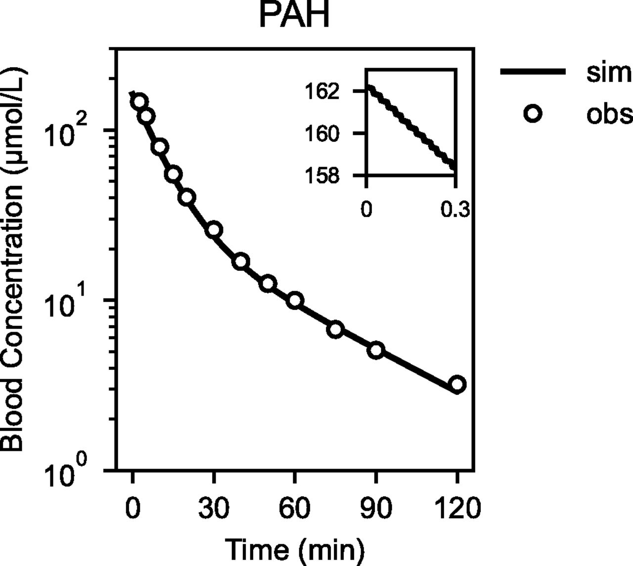
Blood concentration–time profile of PAH after intravenous administration. The observed data from Fagan et al. (1982) (open circle) and the simulated result obtained using the two-compartmental hybrid automaton (solid line) are shown.
In Example 2, we constructed a three-compartmental model to investigate the applicability of hybrid automata to the analysis of drug elimination from the liver. When the parameters in the model were optimized using the blood concentration–time profile of propranolol after intravenous administration, 72.4 liters, 101 l/min, 0.211, 0.0749, 0.00964, and 0.00282 minute−1 were obtained for Vcent, CLint,h, kc2d,1, kd2c,1, kc2d,2, and kd2c,2, respectively, indicating that fu,bCLint,h became about 16 times higher than the hepatic blood flow rate (1.45 l/min). The steady-state distribution volume Vd,ss was estimated to be 7.5 l/kg, which was 1.2 times the value (6.1 l/kg) calculated from the blood concentration data (Fagan et al., 1982). The simulated blood concentration of propranolol showed separate distribution and elimination phases and closely reproduced the observed values (Fig. 4).

Blood concentration–time profile of propranolol after intravenous administration. The observed data from Prescott et al. (1993) (open circle) and the simulated result obtained using the three-compartmental hybrid automaton (solid line) are shown.
When a saturable or an inhibitory component were incorporated in the model of Example 1 simplified by deleting the distribution compartment, the nonlinearity and DDI of virtual drugs could be simulated (Supplemental Information 1; Supplemental Figs. 2 and 3). The way to deal with nonlinearity and DDI in hybrid automata was not so much different from that in traditional pharmacokinetic models.
These results suggested that the hybrid automata are applicable to describe the renal/hepatic clearances limited by the blood flow rates, nonlinearity, and DDI.
Tube Flow
To characterize the tube flow constructed using hybrid automata, we simulated several types of one-dimensional flow after instantaneous injection of a virtual drug. In the model of flow with convection, the drug flowed without diffusing back and forth (Supplemental Movie 1, red), whereas, in the model of flow with both convection and diffusion, the drug flowed with symmetrical diffusion (Supplemental Movie 1, blue). In both types of flow and for all cases of N = 5, 10, and 20 (τf = 0.02, 0.01, and 0.005 minute, respectively), the peaks of drug concentration transited at exactly 0.1 minute (Vtube/Qf). The transit time of the fastest drug was 0.05 minute for N = 5, 10, and 20. Therefore, in the flow models using hybrid automata, the velocity of drug movement was independent of N and τf. On the other hand, the tank-in-series model using ODEs behaved more like a wave than a flow (Supplemental Movie 1, green). The drug dispersed faster from upstream to downstream in the early phase (<0.03 minute) but stayed longer in the downstream in the later phase (>0.140 minute) compared with the two hybrid automata. When the maximum regional concentration was compared by dividing the tube into five regions, the tank-in-series model with low clearance showed 0.363 times lower concentration in region 2 and 0.193 times lower in region 5 relative to the concentration detected in the hybrid automaton with convection when N = 5 (Supplemental Table 11). When we compared the regional cleared amounts, the tank-in-series model produced almost the same result as the hybrid automaton with convection in the case with low clearance. In the case with high clearance, the tank-in-series model underestimated the cleared amount in the upstream region and overestimated that in the downstream region compared with the two hybrid automata, giving concentration of 0.777 times in region 1 and 23.6 times in region 5 relative to those produced by the hybrid automaton with convection when N = 5 (Supplemental Table 12). These results suggested that the tank-in-series model produces dispersed and underestimated concentrations with longer residence in the downstream region even if the whole organ availability is adjusted by N. However, investigations for individual drugs will be needed to allow discussion and evaluation of the risk of using simulation results based on such underestimated concentrations as a virtual clinical evidence.
Body Fluid
We simulated the body fluid volume–time profiles on a virtual day based on the hybrid automata constructed by connecting several parts (Fig. 5). After drinking or eating, the total fluid volume in each intestinal region increased then decreased over time, and the time to maximum volume in each region increased as fluid progressed through the digestive tract. The maximum amount of water was also calculated to be as upper jejunum > lower jejunum > upper ileum > lower ileum, reproducing the phenomenon that water is absorbed as it transits the gut. The movement of water in the digestive tract is also shown in Supplemental Movie 2. Although 200 ml of the water drunk did not reach the end of the ileum, water drunk with meals could reach the last compartment of the ileum because of the water-retaining effect of food residues; this was absorbed in the large intestine. The water balance in the body was defined as the difference between water gain caused by drinking and eating, and water loss caused by urination, defecation, and insensible water loss. The volume of interstitial fluid fluctuated with the water balance (Fig. 5). During the 9-hour overnight period when water could not be drunk, the interstitial fluid volume continued to decrease, whereas urine accumulated in the bladder. However, the urine production rate gradually decreased as the interstitial fluid decreased. The gallbladder was modeled to begin to contract 7.5 minutes after food intake and to replenish 45 minutes later. By the time the gallbladder finished replenishing, most of the stomach contents had been emptied. The hepatic blood volume remained constant, whereas the urine volume periodically rose and fell in the same region and decreased because of water reabsorption through the tubules. The rate of urine reabsorption in the collecting duct was adjusted for the change in the interstitial fluid volume. These results suggested that hybrid automata are applicable to the simulation of the fluid transition and daily water balance in a human body.

The simulated fluid volume–time profiles in the body on a virtual day, simulating the changes in the fluid volume in the body. For upper jejunum, lower jejunum, upper ileum, and lower ileum, the sums of the volume in each region are plotted. asc, ascending colon; bduct, bile duct; dsc, descending colon; duo, duodenum; fhb, flowing volume of hepatic blood; gbd, gallbladder; glm, glomerulus; hb-inlet, hepatic blood inlet; hb-outlet, hepatic blood outlet; if, interstitial fluid; lw-ile, lower ileum; lw-jej, lower jejunum; pv, portal vein; rb, renal blood; rec, rectum; ru, renal urine; stm, stomach; tsc, transverse colon; ubd, urinary bladder; up-ile, upper ileum; up-jej, upper jejunum.
When the body fluid model constructed was applied to describe the disposition of 5-ASA and Ac-5-ASA, the blood concentration–time profiles after oral administration of various formulations were successfully reproduced (Supplemental Information 8; Supplemental Fig. 13; Supplemental Table 13). And then, when the disposition of a virtual compound and its glucuronide that undergoes enterohepatic circulation was simulated using the body fluid model, the blood concentrations of the parent and conjugated compounds were fluctuated after taking meals (Supplemental Information 9; Supplemental Movie 5). These analyses suggested that the body fluid model defined by hybrid automata can be used as a drug container for pharmacokinetic analysis.
Discussion
In the present study, we introduced hybrid automata that handled both discrete and continuous processes for flow modeling. The blood concentration–time profiles of PAH and propranolol after intravenous administration were successfully reproduced by the hybrid automata. The nonlinearity and DDI could be dealt with in hybrid automata as well as the traditional pharmacokinetic models. A body fluid model coordinated various flows in a human body with scheduled daily activities and could be used as a drug container to describe formulation-dependent disposition of 5-ASA and enterohepatic circulation of a virtual drug. These results have demonstrated a high versatility and a wide range of applicability of hybrid automata to various pharmacokinetic analyses.
Because the flow models by first-order kinetics in ODEs focus only on the relationship between input and output concentration, they are unaware of any logical inconsistency inside the organ. For example, suppose the simulation using a model that includes a six-compartment kidney (Burt et al., 2016), a five-compartment liver (Watanabe et al., 2009), and a seven-compartment gastrointestinal tract (Yu and Amidon, 1999), all defined by the first-order kinetics in ODEs. When this model was simulated using a step size of 0.001 hour, the simple calculations are as follows: the blood volume in the kidney is 29.4 ml, so the volume of each of six compartments becomes 4.9 ml. Because the blood flow rate in the kidney is 1250 ml/min, 75 ml of blood should pass through during each step. Although 75 ml of blood is equivalent to 15 times the volume of each compartment, the drug can only move to the next compartment during one step. Similarly, because the blood volume and flow rate in the liver are 194.4 ml and 1450 ml/min, respectively, 2.2 times the blood volume of each compartment should pass through during one step. Yu and Amidon (1999) defined the first and seventh compartments of the gut model as stomach and colon, respectively. In this case, a small amount of drug administered into the stomach can arrive at the colon six steps after administration. If the step size is set to 0.001 or 0.0001 hour, the drug starts to arrive at the colon in 21.6 or 2.16 seconds, indicating that the velocity of the fastest fluid is 13.9 or 139 cm/s if the length of the small intestine is 300 cm. The velocity of an object in a system must be determined by the system. It is logically unacceptable that the velocity of drug movement depends on the step size set by a model user or adjusted by an ODE solver.
It is difficult to model a whole human body using flow models in PDEs because of their excessive calculation costs. For example, suppose the case where the transition of liquid in the small intestine was discretized to the same extent as the renal blood flow. In our model, τrb was set to 0.004 minute, and the transit time through the small intestine was 180 minutes. If the model was discretized so that the fluid could move one compartment every 0.004 minute, the number of compartments required for the small intestine would be 45,000, which is 1500 times that required for our body fluid model. If the discretization levels were the same extent as those for clearance (ODEs), the number would become much larger. Such a model would provide an unnecessarily high resolution of time and space, and it would take too long to obtain the simulation results.
Hybrid automata incorporating various intervals for multiple recursive equations could avoid the problems of the above flow models in ODEs and PDEs. Because the drug flowed in every interval according to recursive equations, the velocity of drug movement was independent of the step size for the ODE solver (Supplemental Movie 1). By fixing the flowing volume to the tube volume divided by the number of compartments, the flowing volume is never larger or smaller than the compartment volume. Because a hybrid automaton can combine multiple flows with different extents of discretization, the intestine was able to save the number of the compartments to be less than 40 and to cooperate with other body parts of higher resolution within a single model (Fig. 5). Under the circumstances when the whole body cannot be simulated by PDE models, a flow model based on the hybrid automata may be an effective option to construct the whole body model as a drug container.
The flow models based on hybrid automata are mathematically related to other flow models (Supplemental Information 10). Roughly speaking, the hybrid automaton incorporating fraction flowed can be regarded as a discrete form of the transition defined by first-order kinetics, and the hybrid automaton with/without incorporating fraction diffused can be regarded as a discrete form of dispersion/parallel-tube model. The well stirred and parallel-tube models are the simplest flow models defined in an ODE and a PDE, respectively, because they can be derived from a one-organ model and a one-dimensional convection-reaction equation, respectively (Rowland et al., 1973; Pang and Rowland, 1977). The organ clearance of the simplest flow model using hybrid automata can be derived from a hybrid automaton with one vertex and expressed by eq. 21:
 where Vf is a flowing volume and τf is a time interval. As with the other simplest models, the one-vertex hybrid automaton is also capable of considering the rate-determining step. Because one vertex does not incorporate axial spreading, the organ availability of this model is equivalent to that of the parallel-tube model when Q = Vf/τf.
The advantage of the hybrid automata with various intervals for multiple recursive equations is that the resolution of a specific part of a model can be adjusted relatively freely while the whole body is being roughly modeled. One of the difficulties in pharmacokinetics is that researchers cannot avoid considering the morphologic and physiologic complexity of the human body because pharmacokinetic phenomena result from the whole body. The method to express a whole body as a rough model with the lower resolution will continue to be important until technologies develop sufficiently. The more deeply that researchers understand the human body and the more rapidly computers can calculate, the higher resolution researchers can use for regions of interest in a body. The hybrid automata will gradually make progress from a coarse model that roughly approximates a whole body toward a fine model that deserves to be called physiologic reality. This is in contrast to the tank-in-series model, in which the number of compartments is determined based on an organ clearance.
The hybrid automata constructed in this study have yet to be refined. In the present study, we simplified many problems, made various assumptions, and omitted important anatomic structures and physiologic functions. More complex and expressive models will be necessary to reproduce the diverse functions of the human body. If blood segregation or enzyme zonation needs to be considered (Cong et al., 2000; Liu and Pang, 2006), the hybrid automata have enough capability for expansion to define a branched flow or a nonuniform distribution of clearance. Because the current solver is required to fix τ values during the calculation, it is necessary to improve the solver to incorporate functions involving changes in τ, such as fluctuations in heartbeat, gastric peristalsis, and interdigestive migrating motor complex (Oberle and Amidon, 1987). Complex modeling requires broad and detailed data. We had to assume arbitrarily the values for many parameters because of the lack of observational data; therefore, it is important to accumulate data to be available for modeling in the future.
In conclusion, we have proposed flow modeling using hybrid automata that could avoid the logical inconsistency observed in the flow expression by first-order kinetics, and that could save the number of compartments by coordinating flows with different extents of discretization compared with a PDE model discretized with a single interval. The preliminary application of this method to several examples demonstrated the high versatility of the hybrid automata in pharmacokinetic analysis. In future, hybrid automata might be useful to develop a more realistic model capable of describing not only pharmacokinetics but also physiology and pathophysiology to allow a better understanding of the human body. The method and the theory in this study will provide a basis for further development.
Authorship Contributions
Participated in research design: Koyama
Conducted experiments: Koyama
Contributed new reagents or analytic tools: Koyama
Performed data analysis: Koyama
Wrote or contributed to the writing of the manuscript: Koyama
Footnotes
- Received August 27, 2020.
- Accepted April 5, 2021.
This work received no external funding. The author declares that there is no conflict of interest.
↵
 This article has supplemental material available at dmd.aspetjournals.org.

Abbreviations
- Ac-5-ASA
- N-acetyl-5-aminosalicylic acid
- 5-ASA
- 5-aminosalicylic acid
- CLint
- intrinsic clearance
- CLorg
- organ clearance
- DDI
- drug-drug interaction
- fd
- fraction diffused
- ff
- fraction flowed
- fu,b
- fraction unbound in blood
- N
- number of compartments
- NM
- Nelder-Mead
- ODE
- ordinary differential equation
- PDE
- partial differential equation
- PAH
- p-aminohippurate
- PS
- permeation clearance
- Qf
- blood flow rate
- τ
- time interval
- τf
- interval of flow
- Vf
- volume of flow
- Copyright © 2021 by The Author(s)
This is an open access article distributed under the CC BY Attribution 4.0 International license.


